Time Series Analysis

Time series analysis is a vital statistical technique for examining data points collected or recorded at time intervals. In R, it involves identifying patterns, trends, seasonality, and cyclical behavior within a dataset. A typical time series analysis begins with data visualization to understand underlying trends, followed by decomposition to separate the data into trend, seasonal, and residual components. Ensuring stationarity is crucial, as non-stationary data can mislead results; this is often checked using the Augmented Dickey-Fuller (ADF) test. If the data are not stationary, differencing is applied to stabilize the mean and remove trends or seasonality. The autocorrelation function (ACF) and partial autocorrelation function (PACF) plots are then used to identify dependencies between observations. These steps help build models like ARIMA (AutoRegressive Integrated Moving Average), which are fitted to forecast future values and gain insights into temporal data behavior. R’s powerful packages, such as forecast, tseries, and ggplot2, make it a preferred choice for comprehensive time series analysis.

Let us explore sample data from base R

data("austres")

This data represents the Quarterly Time Series of the Number of Australian Residents

library(dplyr)

## 
## Attaching package: 'dplyr'

## The following objects are masked from 'package:stats':
## 
##     filter, lag

## The following objects are masked from 'package:base':
## 
##     intersect, setdiff, setequal, union

glimpse(austres)

##  Time-Series [1:89] from 1971 to 1993: 13067 13130 13198 13254 13304 ...

library(tseries)

## Registered S3 method overwritten by 'quantmod':
##   method            from
##   as.zoo.data.frame zoo

my_series <- ts(data = austres,start = 1971,end = 1993,frequency = 4)
my_series

##         Qtr1    Qtr2    Qtr3    Qtr4
## 1971 13067.3 13130.5 13198.4 13254.2
## 1972 13303.7 13353.9 13409.3 13459.2
## 1973 13504.5 13552.6 13614.3 13669.5
## 1974 13722.6 13772.1 13832.0 13862.6
## 1975 13893.0 13926.8 13968.9 14004.7
## 1976 14033.1 14066.0 14110.1 14155.6
## 1977 14192.2 14231.7 14281.5 14330.3
## 1978 14359.3 14396.6 14430.8 14478.4
## 1979 14515.7 14554.9 14602.5 14646.4
## 1980 14695.4 14746.6 14807.4 14874.4
## 1981 14923.3 14988.7 15054.1 15121.7
## 1982 15184.2 15239.3 15288.9 15346.2
## 1983 15393.5 15439.0 15483.5 15531.5
## 1984 15579.4 15628.5 15677.3 15736.7
## 1985 15788.3 15839.7 15900.6 15961.5
## 1986 16018.3 16076.9 16139.0 16203.0
## 1987 16263.3 16327.9 16398.9 16478.3
## 1988 16538.2 16621.6 16697.0 16777.2
## 1989 16833.1 16891.6 16956.8 17026.3
## 1990 17085.4 17106.9 17169.4 17239.4
## 1991 17292.0 17354.2 17414.2 17447.3
## 1992 17482.6 17526.0 17568.7 17627.1
## 1993 17661.5

library(ggplot2)
library(forecast)
 autoplot(austres) +ggtitle("Number of Australian Residents from 1971 to 1993")

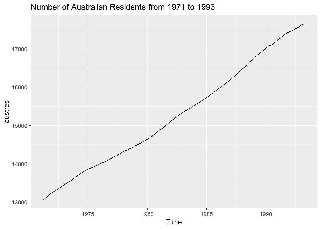The plot indicates that there was a significant increase in population from the year 1971 to 1993.

Decompose the time series

stl_result<- stl(austres,s.window = "periodic")
autoplot(stl_result)

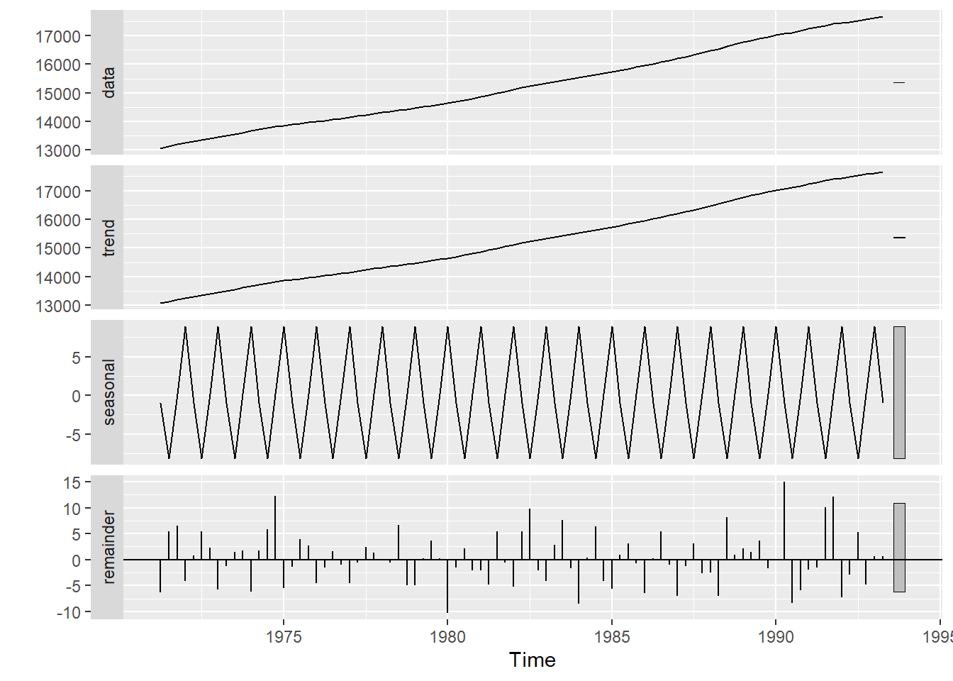
• S.window controls how fast the seasonal effects can change overtime.
  • setting s.window = periodic forces seasonal effects to be identical across the year.
• t.window controls how fast the trend can change overtime.

Stationarity check

Using the Augmented Dickey-Fuller(ADF) to check if the series is stationary.If not ,we difference the data.

• If P-value > 0.05 , the series is non-stationary

adf.test(austres)

## 
## 	Augmented Dickey-Fuller Test
## 
## data:  austres
## Dickey-Fuller = -2.5512, Lag order = 4, p-value = 0.3493
## alternative hypothesis: stationary

diff1 <- diff(austres,differences = 1)
adf.test(diff1)

## 
## 	Augmented Dickey-Fuller Test
## 
## data:  diff1
## Dickey-Fuller = -1.9115, Lag order = 4, p-value = 0.6125
## alternative hypothesis: stationary

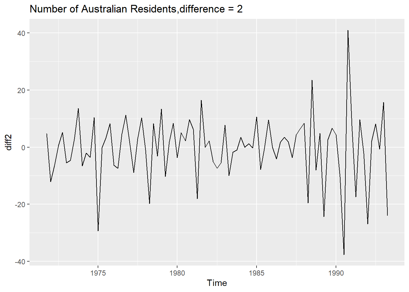
diff2 <- diff(austres,differences = 2)
adf.test(diff2)

## 
## 	Augmented Dickey-Fuller Test
## 
## data:  diff2
## Dickey-Fuller = -4.6107, Lag order = 4, p-value = 0.01
## alternative hypothesis: stationary

autoplot(diff2) +ggtitle("Number of Australian Residents,difference = 2")

Fitting an ARIMA Model

library(forecast)
fit <- auto.arima(diff2)
summary(fit)

## Series: diff2 
## ARIMA(0,0,1)(1,0,0)[4] with zero mean 
## 
## Coefficients:
##           ma1    sar1
##       -0.6051  0.1921
## s.e.   0.0974  0.1075
## 
## sigma^2 = 99.75:  log likelihood = -322.93
## AIC=651.86   AICc=652.15   BIC=659.26
## 
## Training set error measures:
##                      ME     RMSE      MAE MPE MAPE      MASE       ACF1
## Training set -0.4756375 9.872263 6.975463 Inf  Inf 0.6951176 0.05213173

The ACF1 value of 0.052 indicates very low autocorrelation in the residuals, meaning this model has done well in capturing the time-series structure. In well-fitted models, residuals should resemble white noise (uncorrelated random errors).

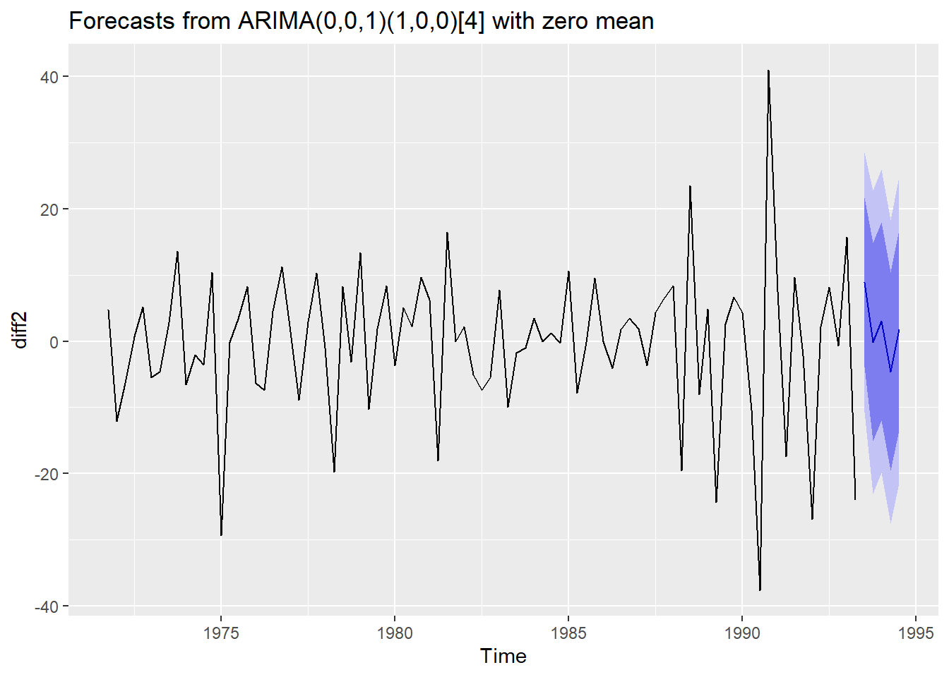
forecasted <- forecast(fit,h=5)
forecasted

##         Point Forecast      Lo 80    Hi 80     Lo 95    Hi 95
## 1993 Q3      8.9173586  -3.882435 21.71715 -10.65824 28.49295
## 1993 Q4     -0.1344916 -15.095304 14.82632 -23.01508 22.74610
## 1994 Q1      3.0164553 -11.944357 17.97727 -19.86413 25.89704
## 1994 Q2     -4.6111419 -19.571954 10.34967 -27.49173 18.26945
## 1994 Q3      1.7133002 -13.448288 16.87489 -21.47435 24.90095

autoplot(forecasted)

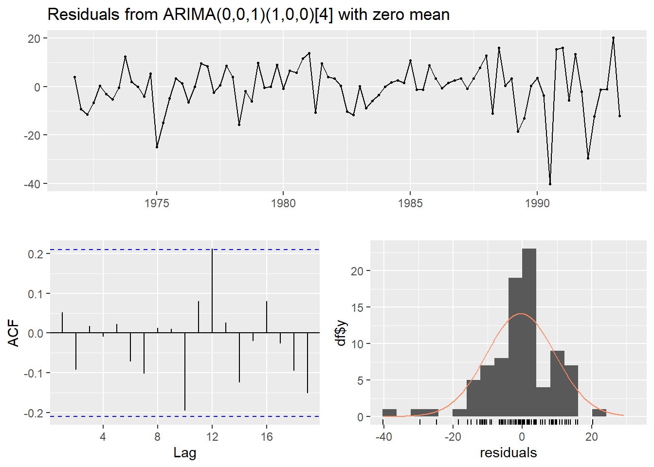
checkresiduals(fit)

## 
## 	Ljung-Box test
## 
## data:  Residuals from ARIMA(0,0,1)(1,0,0)[4] with zero mean
## Q* = 2.6276, df = 6, p-value = 0.8539
## 
## Model df: 2.   Total lags used: 8

• The residuals show no major patterns or autocorrelation, which suggests the model fits well.
• The residuals are roughly normally distributed, which supports the model’s adequacy.